Newsroom

Overview

Diversification is generally understood, but the math is often lost on the less informed. This installment attempts to explain the math involved and point out the flaws in some “rule-of-thumb” approaches or, perhaps even more flawed, the “look-through approach.”

Some History

Several hundred years ago, groups of intelligent homeowners realized that fire was a major threat to their overall welfare and formed “associations.” One of the first in the United States was founded by Ben Franklin:

“In 1752, Benjamin Franklin and his fellow firefighters founded The Philadelphia Contributionship, the longest tenured insurance company in the country”¹

The associations worked perfectly until they did not. The underlying problem was that the diversification was illusory. Because of antiquated building codes and the lack of firewalls, when one home caught fire, all the neighboring homes did as well. Unfortunately, this pattern was repeated in many of the world’s great cities, such as the Great Chicago and London fires, and during World War II with Tokyo, Dresden, Hamburg, and a slew of other cities.

Table I: Hypothetical loans

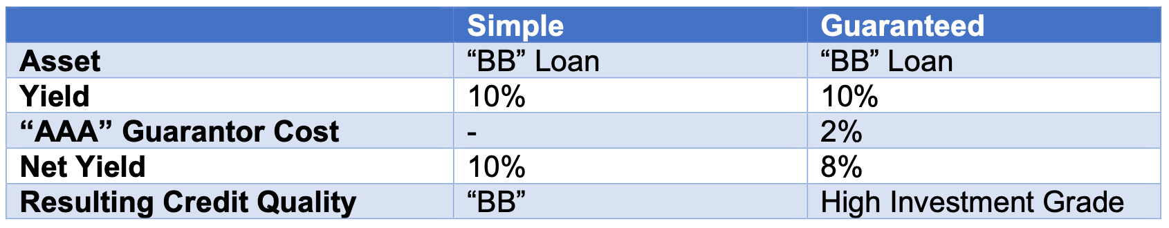
If the guarantee is the equivalent of “hell or high water” (i.e., no room for adjustments), then the Guaranteed Case should warrant a “AAA.” The problem with the “Guaranteed” case is the cost and availability of a guarantee.

Now, let’s evaluate the case of a portfolio of “BB” rated loans, whereby the portfolio is diversified—that is, we do not have the aforementioned household fire insurance problem. Given the notion that a rating is an indication of the probability of default “PD” (or the estimated loss “EL” for some rating firms), the next step is to work out the math for determining the PD or EL.

An easy way to start is to use a small portfolio—in this case, only three uncorrelated loans with credit quality at the “BB” level. Below is a summary of the characteristics of that portfolio.

Table II: Portfolio summary

The first step is working out the various scenarios of default versus non-default. As can be seen in Table III below, in Scenario 1, we assume a default (“D”) for each of the three assets, and on the right side of the chart, a “1” below the number of defaults combinations of “3.” As can be seen in the last row, in only 1 scenario out of 8 is there a triple default, in 3 scenarios out of 8 are there double defaults, in 3 scenarios out of 8 are there single defaults, and in 1 scenario there is no default.

Table III: Default scenarios

The next step is determining the probability of each scenario, which is not equally likely to occur due to the low one-year probability of default given in Table II (2%).

This step is less intuitive, but the sum of the probabilities must equal 100%. The appendix lists the formula for calculating the exact probability, but the results are listed below in the highlighted row.

Starting with Combination 0 (0 defaults), the Income was $10, and the Gain was $10.

With Combination 1 (1 default), the Income is only $6.67. We recover 50% of the $33.33 investment in the defaulted asset for a total Asset Recovery of $16.67. Asset non-recovery ($16.67) minus income yields a Loss of $10. Multiplying the Loss by the Probability yields the results in row 5.

Table IV: Expected loss calculation

Key point: Hence, the EL is reduced from 1% for a portfolio with 1 asset to approximately 0.62% for a portfolio with 3 assets. With 5 assets, the EL is reduced to 0.24%. With 10 assets, the EL is 0.04%.

One might ask why there is a benefit of diversification. The answer probably lies in the fact that the return of the performing assets lessens the sting from any defaults. In fact, one could argue that most financial institutions are built on the concept, whereby banks, insurance firms, brokerage firms, asset managers, and clearing firms all rely on diversification for risk management.

Back to our example: with the addition of more diversified assets, longer holding periods, and some subordinated capital, the EL plunges and credit quality improves. In the case of middle market loans, the typical asset quality is “BB,” the typical subordinated debt is 10%, and the typical rating on the senior debt is “BBB+,” and in some cases, “A-.”



To reiterate, the steps for calculating EL are:

1. Identify various scenarios
2. Identify default combinations
3. Calculate the probability of each combination
4. Calculate cash flows and LGD for each combination
5. Multiply the probability and LGD for each combination to determine the total EL
6. Match the EL to the related rating

Appendix

The formula for determining the Probability of each Combination is listed below²:

For the first Combination, the number of instances of one default is 1. The probability of default is 2% raised to the power of 1 for one defaulted asset. Hence, the formula is as follows:

Px = 1* .0189^0*q^(n-x)

Px = 1* 1 *  q^(n-x)

Px = 1*    .9811^(n-x)

Px =      .9811^(3-0)

Px =      .9811^(3)

Px =      94.44%

Sources

[1] https://1752.com/about-us/history/

[2] https://en.wikipedia.org/wiki/Binomial_distribution

[Table I-IV] https://chatgpt.com/share/67094930-4afc-8011-98ba-70f585d1e175